Ambiguity Diagram Computer
Introduction
An echolocation system involves the transmission of a known signal, detection of an echo reflected from some target, and a comparison of the returned echo with the transmitted signal. Information about the target is contained in the difference between the transmitted signal and the echo. For example, range is proportional to the time elapsed between the transmission of the signal and the reception of the echo; information about velocity is represented by a change in frequency and duration of the echo.
To obtain the best performance from an echolocation system it is necessary to maximise the signal to noise ratio of the returned signal and to be able to distinguish the signal from background clutter. If the transmitted signal were a pure sinewave this could be done by using a narrow bandwidth filter on the receiver, tuned to the frequency of the transmitted signal. The filter should not be too sharply tuned however since echoes from moving targets could have doppler shifts greater than the bandwidth of the filter and would therefore not be detected (for a moving target indicator the converse technique is used - a narrow bandwidth band reject filter to remove all echoes from stationary targets, which have no doppler shift). An optimally narrow filter could be used if the filter were scanned until an echo was detected, which also provides a measure of the doppler shift and therefore the target velocity. However, the target must be present for long enough for the filter to find it, and if the filter is scanned then its passband becomes a line spectrum with the lines spaced at the scan frequency of the filter. Only slow scan rates may therefore be used, and the narrower the filter bandwidth the slower the scan rate must be. The effect is directly analogous to the broadband mode of the super-het. bat detector with a swept local oscillator.
Alternatively, it would be possible to use a bank of filters each tuned to a different frequency, but this involves considerable increase in receiver complexity.
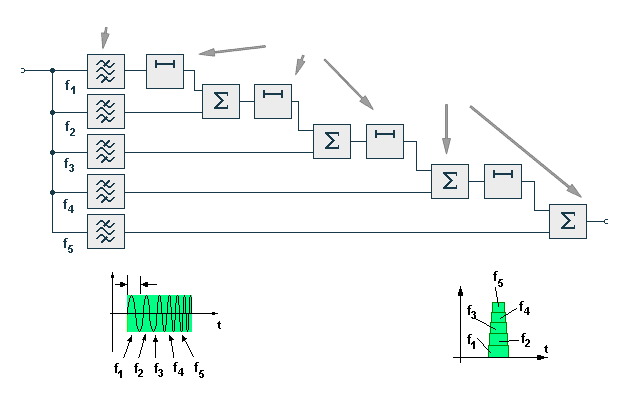
image is available under the GNU Free Documentation License, and the
Creative Commons Attribution-Share Alike 3.0 Unported license, additional terms may apply)
A matched filter for a pulse of this type could be constructed from a tapped delay line and a set of narrow bandpass filters as shown. Each tap on the delay line is connected to a filter, the longest delays corresponding to the lowest frequencies and the shortest delays to the highest frequencies. The delayed and filtered components are then summed to produce the compressed output signal. The centre frequencies of the filters and the time delays can be so chosen that the outputs will occur simultaneously. The output of the matched filter will therefore be a pulse of the same bandwidth as the original signal, but of a shorter duration. It might appear that a great deal of complexity could be avoided by transmitting a shorter pulse in the first place, but it is difficult to transmit high energy levels in a short duration pulse since the peak amplitude that can be handled by the transmitter is limited. To a certain extent resolution can be improved by increasing the number of filters and tuning them more sharply. Increase in resolution is limited however since very sharply tuned filters tend to ring, thus increasing the duration of the summed signal. In addition there will be interference between the outputs of the different filters resulting in the production of sidelobes. The best resolution and accuracy that can be obtained is a function of the signal structure.
Correlation and Fourier techniques allow the synthesis of matched filters for any kind of realisable signal. Although working in the time domain and frequency domain respectively both these techniques are very closely related.
Fourier theory states that any repetitive waveform is the sum of a series of harmonically related sinewaves, the fundamental of the series being the repetition frequency of the waveform. The signal is defined by the phases and amplitudes of the harmonics. The phase may be specified as a phase angle or the harmonic component may be considered as the sum of a sine and a cosine component. As the repetition frequency decreases the harmonic components will come closer together until, in the limiting case of a single event, the spectrum will be continuous.
Sinewaves possess the property of orthogonality. This is shown
in the equations:-
Eq 1. The orthogonal property; the product of any two harmonics has a zero average
If two sinewaves of different frequency, 2πn and 2πm are multiplied and integrated over the repetition period, T, of their common fundamental (in the case of harmonically related sinewaves) or infinity (in the case of non-harmonically related sinewaves), then the value of the integral will be zero. Similarly the integral of the product of a sinewave and a cosinewave of any frequency will be zero. The integral will only have a non-zero value for the product of two sinewaves or two cosinewaves of the same frequency.
Eq 2 The square of any sinusoid is always positive.
The exception to this occurs when the value of n is zero in which case the product of the two sinewaves will be zero while the product of the two cosinewaves will be one.
If we wish to measure the amplitude of the sine components of a waveform at a certain frequency it is necessary to multiply the signal by a sinewave of that frequency and integrate the product. If the process is repeated with a cosine of that frequency then the amplitude of both sine and cosine coefficients, and therefore phase and amplitude, will have been determined. By repeating the process at different frequencies, the entire spectrum of the signal can be determined.
It is not necessary to multiply the waveform by a single sinewave at a time. A number of different sine and cosine waves may be combined, and the waveform multiplied by the composite signal. The value of the resulting integral will be the sum of the integrals that would have been obtained using individual sinewaves. The more sinewaves that the waveform has in common with the composite test waveform the greater will be the amplitude of the resulting integral, and the greatest amplitude will be obtained when the two signals are identical. This value therefore represents a measure of the similarity of the two waveforms.
In practice it may not be easy to multiply the two waveforms together in this way due to the difficulty in aligning them in time. If the two waveforms are offset and multiplied and then one is shifted slightly in time with respect to the other and the integral of their products plotted as a function of the time shift, then the maximum of this function will occur at the moment when the two functions were exactly matched in time. This process is referred to as correlation and the resultant function is the cross-correlation function of the two signals.
The auto-correlation function of a signal (i.e. the cross-correlation function of a signal with itself) is the same as the output of a matched filter for that signal. It is therefore possible to use the correlation process in a receiver in the same way as a matched filter is used. A replica of the transmitted signal is stored in the receiver and the returning signal is correlated with the replica as it arrives. The time delay is produced by the time taken for the signal to travel to the target and back. If a small amount of the transmitted signal is leaked into the receiver during transmission then there will be two peaks in the output, one for the transmitted signal and one for the echo, and the separation of these corresponds to the range of the target.
When designing a signal for use in an echolocation system it is desirable to find one which will have an auto-correlation function with as narrow a peak as possible, thus reducing the error with which time delay can be measured. It is also necessary to minimise the size of any sidelobes in the vicinity of the main peak, so as to be optimise the range resolution of the system. The auto-correlation function of the signal only represents the output of a receiver in response to an input which is an identical copy of the stored signal, i.e. an echo from a stationary point target in a non-dispersive medium. If the echo is distorted, then in any way then the cross-correlation function between the stored signal and the echo will be degraded with respect to the auto-correlation function. The most common form of distortion (assuming a non-dispersive medium) is the change in frequency produced by the doppler effect when a target is moving. If we wish to assess the usefulness of a particular type of signal for measuring the range or velocity of a target then we may assemble the cross-correlation functions of the signal with doppler shifted versions of itself, thus producing a three-dimensional graph with horizontal axes of time delay (range) and doppler shift (velocity). If phase can be ignored, as is often the case, then the squared envelope of this function can be plotted, in which form it is known as the ambiguity diagram for that signal.
Woodward (1953) described the narrowband ambiguity function as:-
ω = 2πf
t = negative of time delay
τ = -(2ω v)/c = frequency shift due to the doppler effect
f = carrier frequency of the signal in radians/second
v = radial velocity of the target = - dR/dt
R = range of the target
s(t)= transmitted or reference signal
c = speed of propagation of the signal
Eq 3 Woodward’s wideband ambiguity function
In this case it is assumed that the velocity of propagation of the signal is far greater than the velocity of the target and that the carrier frequency is large compared to the change in frequency due to the doppler effect. For radar these assumptions are usually valid and the doppler shift may be considered to be a simple shift of the total spectrum. For sonar these assumptions do not hold and the doppler shift must be recognised as a compression or expansion of the time axis.
The change in frequency will therefore be a proportional change and not a simple offset. The wideband version of the ambiguity function has been described by Kelly and Wishner ( ) and has been used by Cahlander (1967) in the analysis of a series of five echolocation pulses of the bat Myotis lucifugus and one pulse of the bat Lasiurus borealis. In this case the formula is :-
α = doppler factor =
v = radial velocity of the target
The factor normalises the energy in the echo.
Eq 4 The wideband ambiguity function
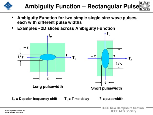
Fig AMB3 Sections through ambiguity functions optimised for measuring range (b) or velocity (a)
The accuracy with which the range can be measured is given by:-
= the echo-delay incrment that can just be discriminated
= the target range increments that can just be discriminated
β = the RMS bandwidth of the system = the energy in the received signal
N0= noise power per unit bandwidth for a real Gaussian noise waveform
E = the total signal energy received
Eq 5 Range discrimination
To obtain an ambiguity diagram with a ridge along the tau-0 axis the signal should have a time bandwidth product of unity. Unfortunately, this leads to severe limitations on the use of these types of signals since the output of the transmitter is usually amplitude limited and as the bandwidth of the signal is increased its duration must decrease, thus reducing the amount of energy that can be transmitted.
To measure the velocity of a target an ambiguity diagram with a ridge running at right angles to that for the range measuring signal is required fig. AMB3 b. In this case the sections through the diagram represent the outputs of a Fourier transform receiver (Bird 1974) which operates on a similar basis to the correlation receiver but in the frequency domain rather than in the time domain. The measure of a target’s velocity can be seen to be independent of the range of the target. The accuracy with which the velocity can be measured is given by:-
δf = frequency increment that can just be discriminated
δv = velocity incrment that can just be discriminated
τ = RMS time duration of the signal
ft = transmitted frequency
Eq 6 Velocity discrimination
An ambiguity diagram of this type will also be produced by a signal with a unity time bandwidth product. The effective duration of the signal in this case will be the bounded by the time for which the target is in the ‘field of view’ of the system.
It can be seen from equation 5 that there is no limitation on the duration of the signal used to measure range, so long as the bandwidth is maintained. Increased power may therefore be achieved by the use of signals with large time bandwidth products. Since accuracy in the measurement of velocity is proportional to the duration of the signal however, this will obviously result in some velocity information being available. In radar systems a common type of signal with a large time bandwidth product is the linear frequency sweep. It can be seen from fig. AMB4 that if such a sweep is shifted in frequency then a shift along the time axis will suffice to provide an almost perfect match with the transmitted signal. The effect of this on the ambiguity diagram is shown in fig. AMB2 c. It can be seen that as the velocity of the target increases a greater time delay is needed before the two signals match and the peak of the correlation function is produced. The width of the peak however remains narrow, i.e. there is still good range accuracy, and the amplitude of the ridge will not fall appreciably for moderate velocities. The signal is therefore said to be doppler tolerant and to produce range-doppler coupling. Although the error in range measured in this way may seem to be a severe disadvantage of this system, this may be resolved either by the use of a second system with a different degree of range doppler coupling or from ^&a priori\& knowledge of the velocity derived for example from range rate measurements.
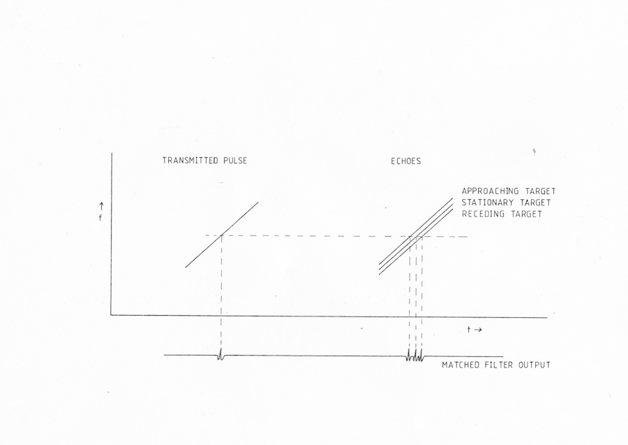
Fig AMB4 Effect of Doppler shift on the response of a linear fm matched filter with approaching or receding targets.
A ridge almost parallel to the velocity axis, while having good range accuracy, will have poor velocity accuracy. Similarly, a ridge skewed almost parallel to the time axis will have better velocity than range accuracy. Any improvement in one, by rotation of the ridge, will result in a corresponding degradation of the other. If it is required to obtain high accuracy in both range and velocity, then a signal whose ambiguity diagram is a single sharp peak is required. A number of problems occur with this type of ambiguity function. In the narrowband case, and generally in the wideband case, the volume of the ambiguity function is fixed, and the height of the central peak is fixed. When this is true, making the central spike thinner must involve an increase in the height of the ambiguity function elsewhere. Klauder ( ) has described signals which have a rotationally invariant ambiguity function, in which the volume removed from the peak is spread in concentric rings around the peak. By suitable design it should be possible to arrange that the rings spread far enough away from the centre, that their height at any point was less than some arbitrary limit. Whether such signals are physically realisable is not certain. A ‘bed of nails’ ambiguity function can also be achieved (Rihazcek ), which consists of an array of thin peaks; this may be useful when ^&a priori\& constraints may be placed on the possible range and velocity of the target so that the multiple ambiguities may be resolved.
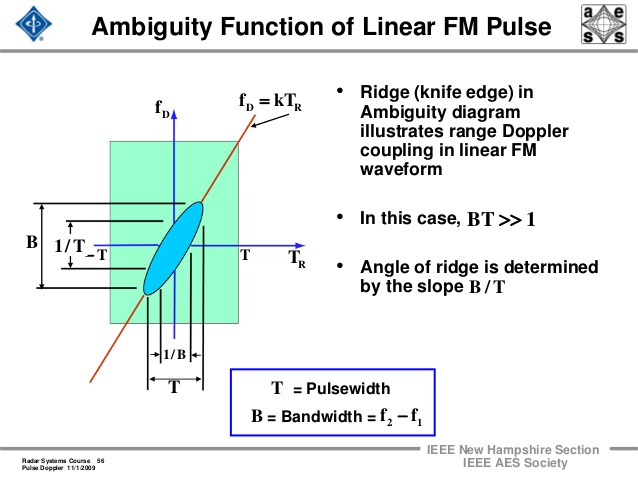
Fig AMB5 Ambiguity function of a linear fm pulse
A further problem concerns the subject of target detection. An ambiguity diagram which is flat everywhere but in the centre, implies that, in a range measuring system, there will be no output from the matched filter in response to echoes from moving targets with a doppler shift and therefore only stationary targets will be detected. Similarly, in a velocity measuring system where the receiver output corresponds to slices through the ambiguity function at right angles to the correlation functions, a response will only occur to targets at a specific range.
The Ambiguity Diagram Computer
The ambiguity diagram may be computed by producing a set of cross-correlations between the signal of interest and energy normalised doppler shifted versions of that signal. To generate such a diagram, it is necessary to a) apply a doppler shift to the signal, b) delay the shifted signal by successive increments with respect to the reference signal, c) multiply the two resultant signals together, d) integrate the product and plot the integral as a function of the time delay. For small doppler shifts little error is introduced if the energy normalisation factor s^1/2 is ignored, and the integral itself may be plotted rather than the squared envelope.
This process may be performed by using a digital computer, either defining the signal as a mathematical expression and evaluating equation 4, or by sampling a real signal through an analogue to digital converter (ADC) and using discrete Fourier transforms (DFTs) in the generation of the correlations.
When using digital techniques, the doppler shift may be produced by varying the sampling rate in the ADC. The problems are that if the signal is to be defined mathematically, then consideration is limited to those signals which are readily amenable to mathematical description, while if analogue signals are used then a large memory is required to store the signals (approx. 300,000 samples per second for signals with a bandwidth of up to 100 kHz) unless they are stored in analogue form outside the computer and re-read for each correlation. While the memory requirements are by no means prohibitive in the light of modern technology, use of micro-computers will be found to be very slow due to the large number of multiplications involved in computing fast Fourier transforms (FFTs) of large samples, while mini-computers are comparatively expensive items of capital equipment.
Mainframe computers could be used if available but tend to be very expensive to use and are unsuited for real-time data acquisition.
An alternative technique would be to use dedicated integrated circuits to calculate the FFTs at high speed. This would make the use of a micro-computer for the task much more practicable, but the cost would still be very high.
Design and Construction
The main requirements in the design of the ambiguity diagram computer were that it should be capable of computing the ambiguity diagrams for real bat signals recorded on magnetic tape, and that the cost should be as low as possible. It was also desirable that it should be possible to run the computer without having to rely on external assistance (e.g. for digitising the signals to be analysed), and that it should be possible at some later date to expand the computer to produce other types of ambiguity diagrams. The low-cost requirement suggested that existing equipment should be used as far as possible.
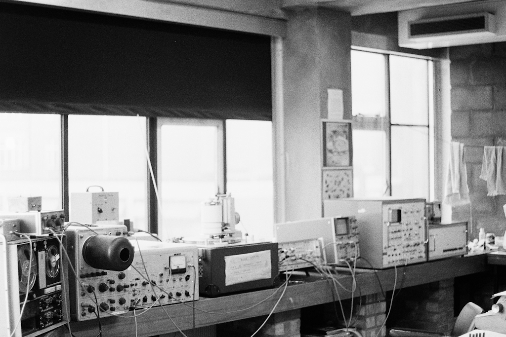
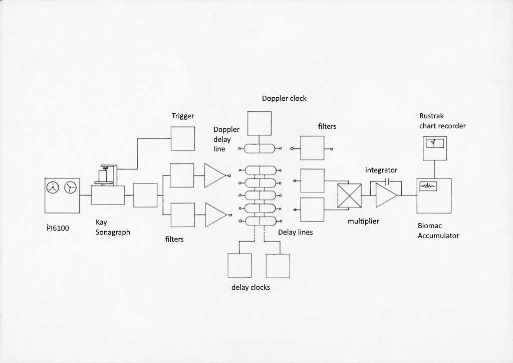
Fig AMB6 Photograph of the complete ambiguity diagram computer and block diagram of the major components. In the photograp, from left to right, the PI6100 instrumentation recorder with a Krohn-Hite bandpass filter on top, Telequipment oscilloscope, Kay Missilyzer sonagraph, Purpose built analogue computer with patch panels, second oscilloscope, Biomac 1000 averaging computer for accumulating results, Power supply and Rustrak y-t chart recorder for plotting completed correlograms.
The complete device is shown in fig. AMB6. It consists of a high speed instrumentation tape recorder, on which the original recordings of the bat’s echolocation signals can be replayed at one eighth or one tenth of the original speed; a Kay Missilyzer Sonagraph type 675 which is used to store the slowed down signal and to replay it repeatedly; an especially designed and built analogue computer for calculating correlation functions and for generating Doppler shifts; a Biomac 1000 averaging computer to store the successive points in each correlation function as they are calculated by the correlation computer; and a Rustrak y-t plotter on which the assembled correlograms are written. Oscilloscopes are used at various points to monitor the amplitudes of the signals so as to ensure that overloading is not producing distortion, and to monitor the progress of the correlation.
To avoid confusion when discussing time delays and time shifts applied to a slowed down signal the terms ‘bench time’ (b.t.) and ‘real time’ (r.t.) will be used to distinguish between the actual times within the computer, and the times scaled by the speed reduction factor of the tape recording. For example, the duration of a bat pulse may be specified as 2938 us in real time or 23.5 ms in bench time.
The sonagraph stores the signal magnetically on a rotating drum, and an optical switch can be adjusted to provide a trigger signal just prior to the occurrence of the signal to be analysed. Also, the drum can be stopped just after the signal and a click can be introduced into the signal by momentarily switching the record head on and off. This click is used as a marker when assembling the final ambiguity diagram. The magnetic drum has two channels, so that it would be possible to generate cross-ambiguity diagrams by recording separate signals on each track. It would however be necessary to ensure that they were closer together than the delay available from the delay lines in the correlation computer. If necessary, this could be done by arranging for one of the heads to be moved to different points on the circumference of the drum.
The sonagraph is also used to produce a sonagram of the signal to be analysed from which it is possible to determine suitable frequency limits for the Krohn-Hite bandpass filter situated between the sonagraph and the correlation computer.
The correlation computer provides increasing time delays for each repetition of the signal, produces a Doppler shifted version of the signal, multiplies the delayed and Doppler-shifted versions, and integrates the product. A single data sample is produced for each repetition of the signal.
A control gate signal is derived from the trigger pulse from the optical switch on the sonagraph. The limits of this control gate are set to occur sufficiently before and after the signal that all delayed and Doppler shifted signals will remain within the period of the control gate. Also, a sufficient gap is left between the leading edge of the control gate and the start of the signal to allow for edge effects when the Doppler shift generator is initiated.
The signal is split into two channels which go to the Doppler shift generator, the incremental delay line, and a fixed delay line which is used to compensate for residual delays in the Doppler shift generator and to ensure that the auto-correlation function has its peak in the centre of the correlogram. One delay line section is devoted to the fixed delay function, while the remaining four sections can be switched between incremental delay and Doppler shift generation. Patchwires are then used to cascade the required number of sections of each type in each of the signal paths.
The delay lines consist of charge coupled, bucket brigade devices. These devices consist of a series of FET switches linking a series of capacitors. A signal at the input is stored as a charge on the first capacitor, and at each clock cycle the charge is transferred one stage along the line, to the next capacitor in the series. Each delay section consists of two delay lines, each of 512 buckets, which may be used singly or in cascade. However, the clocks for each pair of delay lines are common to reduce cross-talk induced clock noise. The delay produced by each delay line is proportional to the period of the clock. Since the maximum signal frequency component is 15 kHz b.t. a minimum clock frequency of 50 kHz was selected, with a maximum clock frequency of 500 kHz, giving a 10:1 range of delays. The delay within each delay line varies between 1.024 ms and 10.24 ms b.t..
The Doppler shift generator uses the same delay lines. In this case however the clock period is changed linearly throughout the period of the control gate. If n delay lines are used then the Doppler shift on the output will not be correct until after 512n clock cycles. This ‘edge effect’ is allowed for when the control gate is positioned around the pulse, so that the signal to be analysed does not enter the delay line until after at least 512n clock cycles. The doppler shift produced is proportional to the number of delay sections and the rate of change of period of the delay line clock.
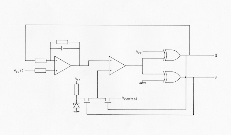
Fig AMB7 schematic of the quadrature VCO
The clocks for both the incremental delay line and the Doppler delay line are of a novel design, in which the clock period is proportional to an external control voltage. The circuit of the VCO is shown in fig. AMB7. When the input to the integrator is high, the output ramps linearly down until it reaches the reference voltage of the comparator. The output of the comparator then goes high causing bar-Q to go low and Q to go high. Q and bar-Q are derived from the comparator output via a matched pair of exclusive-OR gates so as to equalise time delays in both paths as these two signals are the bi-phase clocks for the delay lines. The bar-Q output is fed back to the integrator, causing the output to rise linearly. The Q and bar-Q signals are also used to switch the reference voltage to the comparator between a fixed level and the control voltage. Since the period of the oscillator is directly proportional to the difference in voltage between the two switching levels, then the period will be proportional to the control voltage. Complementary transistor drivers are used to buffer the Q and bar-Q clock signals.
The control voltages for the incremental delay lines are provided by a 10-bit digital to analogue converter, driven by a 10 bit binary counter which is incremented by the trailing edge of the control gate. This provides 1024 discrete control voltages, and hence 1024 points in each correlogram.
For the Doppler shift generator, the control gate is used as the input to an integrator, providing a linear slope throughout the period of the control gate. The integrator is held in a reset state throughout the rest of the cycle. The time constant of the integrator is adjustable in two ways. The capacitor is switchable, so that it is possible to change the number of delay line sections being used without altering the Doppler shifts generated. The Doppler shifts are incremented at the end of each correlogram, when a four-bit binary counter is incremented, which controls a 16:1 analogue multiplexer. The multiplexer selects the resistive element of the integrator from a bank of sixteen preset potentiometers.
The delay in the fixed delay line is controlled by a CMOS VCO, the frequency of which is adjustable from the front panel of the computer.
The output from each of the three banks of delay lines are filtered by 15 kHz low pass, four pole Tchebysheff filters with 1dB of ripple in the pass band.
The delayed and Doppler shifted signals are multiplied using a balanced modulator, with both input signals being monitored on an oscilloscope to ensure that they are not large enough to cause distortion in the modulator. The output of the modulator is then integrated and buffered, with an adjustable time constant in the integrator to allow for variation in the signal durations. The integrator is held in a reset state at all times except for the duration of the control gate.
The Biomac 1000 averaging computer is set to sample the output of the correlation computer at the end of the control gate. When 1000 samples have been taken an end of cycle signal is returned to the correlation computer, which is used to reset the incremental delay counter, and to increment the Doppler shift counter. The Biomac is also capable of writing the assembled correlogram to the Rustrak y-t plotter. In automatic mode the complete set of correlograms can be produced in this way with no need for intervention from the operator, or each correlogram may be produced separately, the computer waiting at the end of each one to be restarted for the next.
The individual correlograms are assembled into the final ambiguity diagram by hand. A decision has to be made however on the relative alignment of the individual correlograms. The alignment depends on the time at which we wish to know the range of the target. For the sake of convenience, we choose to measure the range when an arbitrary point near the centre of the pulse reaches the target. To determine the necessary alignment for this assumption it is necessary to add a marker to the signal in the form of a brief click. This is done by switching the record head of the sonagraph on and off with the drum held stationary just after the signal to be analysed. Since the computer is normally set up to generate negative Doppler shifts (i.e. corresponding to a receding target) then the alignment of the delayed click with the Doppler shifted click will occur before the alignment of the centre of the Doppler shifted pulse with the delayed pulse, by an amount equal to the time delay between the pulse centre and the click multiplied by the Doppler shift. The matching of the clicks is marked on the correlogram with the highest Doppler shift by switching the input to the Biomac to a 9 V source for one sample period when the clicks are seen to be aligned on the oscilloscope monitoring the inputs to the multiplier. When aligning the correlograms the peak of the zero Doppler correlogram is known to lie on the tau-zero axis. The maximum Doppler shift correlogram is aligned by locating the marker blip to the left of the tau-zero axis by a time equal to the centre-pulse to marker distance times the Doppler shift. Intermediate correlograms are then fitted by interpolation such that the ends of the correlograms are aligned.
Calibration of the correlation computer is done whenever the Doppler settings are altered, and the time base is calibrated for every ambiguity diagram. The time base is calibrated very simply by connecting the input to the correlation computer to a sinewave signal generator set to a frequency of 2 kHz, and with the frequency accurately measured with a frequency meter. The auto-correlation function of a sinewave is a sinewave of the same frequency, and therefore plotting the auto-correlation function of the test signal provides an accurate timebase.
Doppler calibration is slightly more complicated. In this case the same input signal is used as for calibrating the time base, but the Biomac is connected directly to the output of the multiplier and is set to read a thousand samples over a period of 40 or 80 ms, with a delay between the start of the control gate and the start of sampling of 10.25 ms. The Doppler shifts for each setting can then be found from the ratio of the frequency of the beat-note to the zero Doppler frequency.
Ambiguity Computer Results
Some ambiguity diagrams of bat pulses produced on the computer are included here to demonstrate the presentation of the output and to show the type of information that can be obtained.
It should be borne in mind that the computer was designed to present qualitative rather than quantitative information. The ambiguity diagrams are plotted on the basis of target position at the time that the centre of the pulse reached the target and are arranged such that a frequency downsweep produces a ridge skewed to the right. For small doppler shifts the ambiguity diagram is reasonable anti-symmetrical about the d=0 axis and therefore only one half of the diagram is plotted. In these examples doppler shifts are all for receding targets.
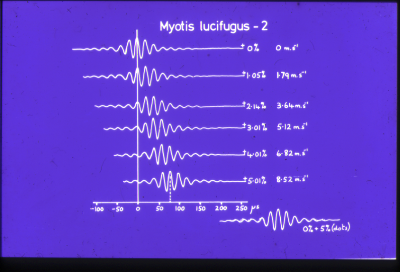
Fig AMB8 Ambiguity diagram of an fm pulse of Myotis lucifugus (after Pye 198 )
A classical fm pulse analysed on the computer has been published by Pye (198 ) and shows the diagonal ridge predicted from theoretical considerations. It can be shown that if the reference point is taken as the time at which the period of the waveform would extrapolate to zero were used instead of the centre of the pulse then the ridge would skew to lie on the tau-0 axis.
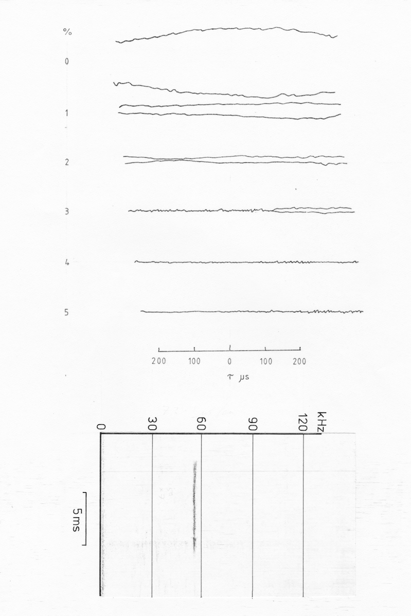
A similar type of pulse from a pipistrelle, Pipistrellus nanus, is shown in fig. AMB9. The recording was made of the bat flying indoors, but there is little evidence of echo in the ambiguity diagram. The pulse has a duration of 1.6 ms and has its main energy centred around 70 kHz. It can be seen that the ambiguity diagram consists of a simple ridge, similar to the Myotis pulse except that at the higher doppler shifts there is a skew in the shape of the peak, in the same direction as the skew of the ridge. The width of the d=0 peak is about 86 us r.t. corresponding to a distance of +/- 15 mm. The width of correlation peaks is measured throughout at the half amplitude point. With a doppler shift of 5% the width of the peak is still only 160 us.
Fig AMB9 Ambiguity diagram of an fm pulse of Pipistrellus nanus
The skew of the ridge is 247 us at 5% doppler, which is equivalent to a distance of 42 mm. This could be reduced considerably by a change of reference point since the theoretical offset with respect to the centre of the pulse for aligning the ridge with the tau-0 axis is 4996 us r.t. (assuming linear period modulation of the signal, and an optimal envelope), while the measured distance from the pulse centre to the pulse zero period extrapolation was 3125 us r.t.. While this is not as close as for the Myotis pulse, it would still reduce the range ‘error’ quite considerably. Also if the doppler shift is high then the relative course of the bat and its target probably has only a small tangential component, in which case range errors will have little effect on the interception ability of the bat. If there is a large tangential component, then there will be comparatively little doppler shift and the bat will achieve close to its best range accuracy.
It must also be remembered that bats frequently use their wings and tail membranes to catch their prey, and this represents a catchment area several centimetres wide.
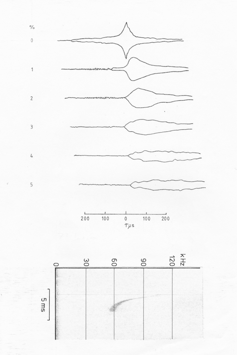
Fig AMB10 Ambiguity diagram of a cf/fm pulse of Rhynconycteris naso
A cf/fm pulse gives a far less impressive type of ambiguity diagram, as shown in fig. AMB10. This short pulse, produced by Rhynconycteris naso has the classical shape of cf/fm pulses, with a constant frequency portion followed by a frequency downsweep. In this case the pulse is quite short, less than 5 ms. Although the cf/fm pulse is traditionally thought of as a doppler pulse with an fm portion thrown in ‘for good measure’, it is strange that a bat should then use such a short duration of pulse.
From the ambiguity diagram it can be seen that the pulse has very poor range measuring properties despite the fm portion and that what peak there is has very poor doppler tolerance. The doppler ridge however appears to have quite good resolution, although the ambiguity diagram as generated here does not show how narrow the ridge actually is. The ambiguity diagram for a pulse of this type would be better if cross-sections could be taken parallel to the tau-0 axis.
It is interesting to compare the skew in the shape of the ridge in the fm pulse of P. nanus with the skew in the (very wide) ridge of the cf/fm pulse. It is probable that this is due to a change in the slope of the frequency sweep since the shift of the main peak is proportional to the slope of the sweep. The presence of different rates of change of period within the sweep would then be expected to first broaden the peak and then, at high doppler shifts, to split into separate ridges. Non-linearity in the rate of change of period within the pulse would have a similar effect. This is very pronounced where the cf changes to fm, and is also just evident at the end of the fm pulse where the dominant energy component occurs.
The sequence of pulses of Pipistrellus pipistrellus (fig. AMB11) were all recorded in the field in early October. The full sequence of pulses starts with the bat using pure cf pulses such as those in fig. AR3 and then, when the target is detected, the bat introduces some fm at the start of the pulse. As it gets closer the amount of fm increases and the amount of cf decreases, until the pulses are pure fm. During the interception buzz the repetition rate of the pulses increases dramatically, and the pulse duration becomes very short. At the end of the buzz there is a pause, presumably while the bat consumes its prey, and then the bat resumes echolocating with hybrid fm/cf pulses.
a
b
c
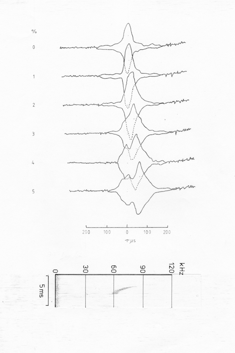
Fig AMB11 Ambiguity diagrams of a sequence of pulses from Pipistrellus pipistrellus (NB now classified as Pipistrellus pygmaeus since 1995) a) cf cruising pulse, b) cf/fm transitional pulse, c) fm/cf pulse just prior to a catch buzz
The first of the pulses illustrated is a typical pipistrelle pure cf pulse with a duration of just under 10 ms at a frequency of 56 kHz. While this frequency is slightly higher than is common for P. pipistrellus in this country there were a number of individuals in this area which used the higher frequency (NB since 1995 P. pipistrellus has been subdivided into two distinct species of which this is P. pygmaeus). The ambiguity diagram of this pulse is just as would be expected, with a large ridge parallel to the tau-0 axis and dropping away rapidly when there is any doppler shift. Again it would be necessary to plot the sections through the ambiguity diagram as a set of functions of doppler shift, to adequately determine the width of the doppler ridge. The tapering of the ridge at either end is due to the comparatively short duration of the pulse.
Once an fm component is introduced into the pulse the d=0 section shows a marked peak with a half amplitude width of 40 us r.t. (= +/- 3.4 mm). The d=0 peak does however have much greater sidelobes than for pure fm pulses.
As the doppler shift is increased the peak is skewed as well as shifted to the right. This is very similar to the fm pulse for P. nanus although much more marked. At still greater doppler shifts the peak disappears leaving just a flat plateau (at least within the area measured) to the right of tau-0.
The next pulse in the series shows a rather unexpected development.
The d=0 section is similar to those of earlier pulses except that the extent and amplitude of the sidelobes has decreased as would be expected in this more strongly fm pulse. However, as the doppler shift increases the ridge splits into two divergent peaks. The main peak moves to the right as would be expected for a downsweep, but the second peak moves very little. It is certainly more doppler tolerant than the main peak.
If the subsidiary ridge were due to an echo then there would a pair of ridges symmetrically arranged either side of the main ridge. A split into two ridges can occur if the pulse contains an upsweep as well as a downsweep but the secondary ridge would then be expected to move to the right of the tau-0 axis. Since this ridge moves very little, if at all, it is probably due to the abrupt termination of the pulse, resulting in a wide bandwidth portion of the signal as the pulse terminates.
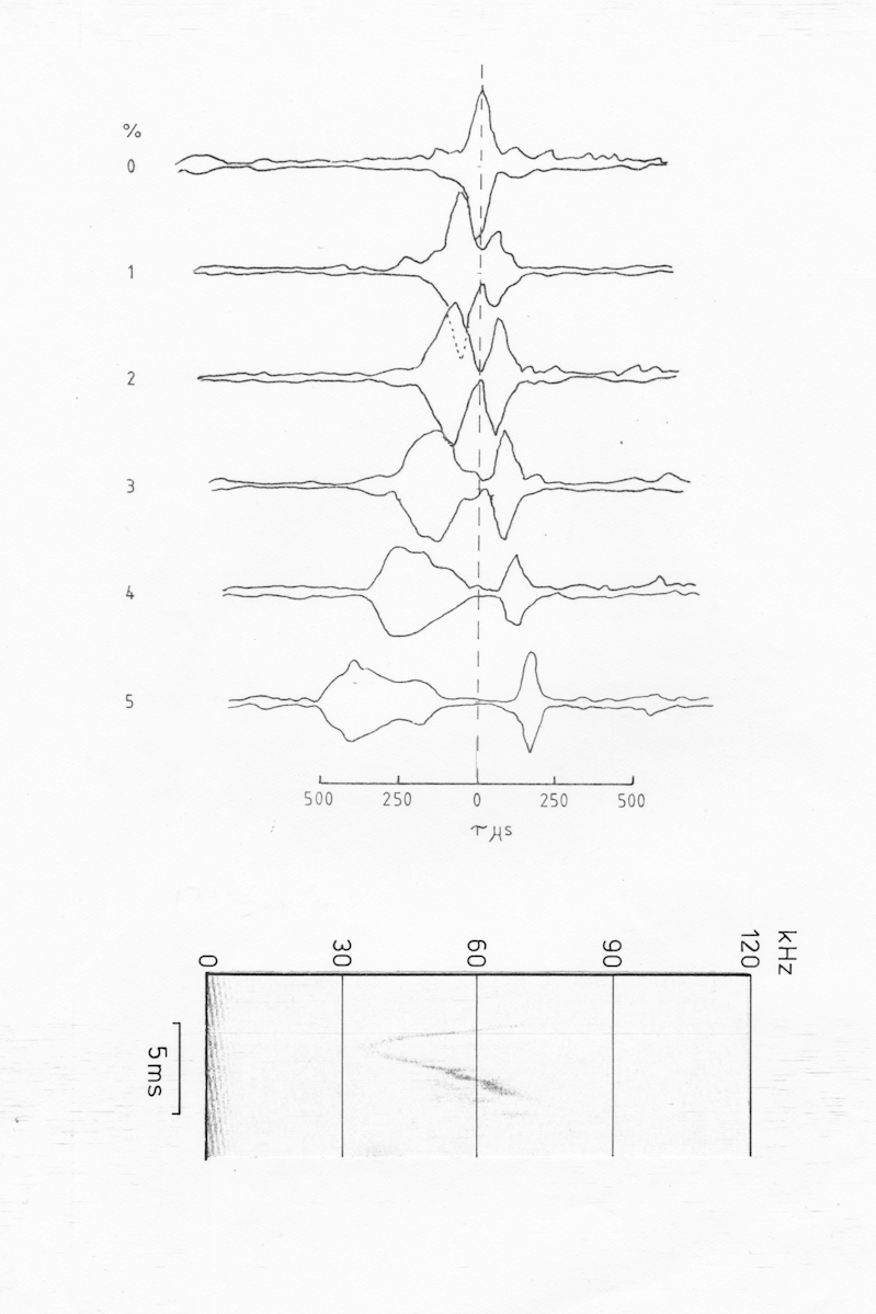
Fig AMB12 Ambiguity diagram of a comples pulse of Natalus stramineus with pronounced up and down sweeps, probably primarily a social call.
The effect of a pronounced upsweep is seen in fig. AMB12, which is of a sound produced by Natalus stramineus when held in the hand. In this case there is a pronounced separation of the two ridges, the downsweep ridge being the narrower and more doppler tolerant, although the upsweep contains greater energy. It is tempting to suggest that such a pulse would be useful in echolocation in a single target environment since it would enable the bat to determine the direction of movement of the target from a single pulse from the order in which the two peaks occur. However, there is no evidence to suggest that pulses of this type are used when the bats are primarily concerned with echolocation, such as when hunting or flying within a confined environment.
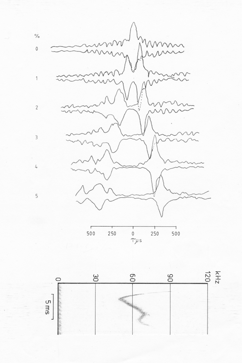
Fig AMB13 Ambiguity diagram of a complex pulse of Natalus stramineus with multiple up and down sweeps
In the case of a more complex pulse with multiple up and down sweeps, fig. AMB13, there is still a pronounced ridge which will provide a considerable amount of echolocation information. In this case however the sidelobes are much more pronounced and complicated due to the interference between different parts of the sweeps. The bat is still able to maintain a general ‘surveillance mode’ of echolocation to warn of approaching dangers even while using the vocalisations for a different purpose.
Discussion
The ambiguity diagram computer is not a universal tool for the analysis of ultrasonic signals. It makes important assumptions about the use of the signals, that they are being used as part of an echolocation system. Also, if we are to attempt to draw conclusions about the echolocation ability of an animal using the signals then we must make the assumption that the animal is using a matched filter, or equivalent receiver.
Simmons ( ) has shown that the autocorrelation function of the echolocation signals of Phyllostamus hastatus show a very good match with its measured echolocation ability in the laboratory. It is not unreasonable to assume that they will be able to perform as well as this in the wild, and that other species will also be able to maximise the information available from the echolocation signals which they use.
As a conservative estimate however we can at least say that the ambiguity diagram sets an upper bound for the performance that can be expected from a bat using a specific type of echolocation signal, on the basis of a single pulse. Ambiguities and inaccuracies may be compensated for by making a priori assumptions about the nature of the target, and by using successive pulses with different characteristics. In order to understand such behaviour however we need to know the basic properties of the different types of signal used and this understanding can be derived from a study of the ambiguity functions of the individual signals.
A functional analysis such as this, rather than a purely descriptive one, may also help to show the relative merits of the vast range of different echolocation signals used by different bats.
The way in which the ambiguity function is presented can have a significant bearing on the amount of information which can be extracted from it. Cahlander (1967) used an isometric display of the function, viewed from above, and with the peaks connected in both doppler and tau directions. This form of display was also used by Beuter ( ), although with more sections and a greater number of lines connecting the separate functions. These forms of display can give a good impression of the overall form of the ambiguity function for the simpler pulses, but they do tend to become confusing when the ambiguity function is more complicated. It is also very difficult to make quantitative estimates from the ambiguity function, although in the case of computer generated functions this information may be separately available to the user.
The technique used here of displaying the envelopes of the individual functions provides a clear display from which measurements may be taken, but involves only a small number of sections through the ambiguity function. In many cases this is adequate, but for some pulses, especially those with a significant cf portion, it would be advisable to generate more sections in the region of the zero doppler section, or to generate cross-sections through the ambiguity function at right angles to the cross-correlation functions. These could then be displayed separately or combined with the cross-correlation functions. The ambiguity diagram computer described here can be modified to work in this way by using the signal from the 1000 step DAC to drive the doppler shift generator, and the signal from the multiplexer to drive the variable delay clock. Alternatively a very high resolution display could be produced by using the DAC type of drive for both the doppler shift and delay clocks, but this would be very time consuming as it takes one revolution of the sonagraph drum (0.8 s b.t.) for each point in the final diagram, plus the time required to plot the successive slices. This time could be reduced considerably if the Sonagraph and Biomac were replaced with a computer equipped with and ADC and DAC to store and replay the signal, and to store and display the final ambiguity function. For the majority of signals however it is unlikely that the increased cost would be justified by the improvement in display resolution.
Interpretation of the ambiguity diagram is not a simple task. The problem posed by range-doppler coupling may seem to be very great when the display is arranged on the basis of range when the centre of the pulse reached the target. It has been shown however that for linear period-modulated pulses the ridge may be de-skewed by changing the frame of reference; in this case by choosing to define range as the distance to the target when the period of the pulse extrapolates to zero. Pye has shown that for a pulse with a rectangular envelope there will be small residual error, but Altes and Johnson show that there is a pulse envelope for which even this error can be eliminated, and that this pulse envelope closely matches that used by Myotis lucifugus in cruising flight. Whether such corrections are of any importance to the bat is a difficult question to answer, but I would suggest that a target of interest to the bat with a high radial velocity, will have a low tangential velocity, and therefore interception is highly likely even if range is not accurately known. On the other hand, if there is a high tangential velocity, making interception more difficult, then the radial velocity will be low and range accuracy will be high.
Resolution and ambiguity are more likely to be of interest to a bat, especially in a crowded environment. For these characteristics the interpretation of the ambiguity diagram is more straightforward. Although the diagram is generated for a single pulse it is reasonable to assume that ambiguities due to second-time-around echoes can be simply resolved by changes in repetition rate, in addition to the fact that atmospheric attenuation will provide a good cut-off from targets beyond a certain distance.
The ability to cope with signal related clutter can also be assessed by means of the ambiguity diagram computer. By using the second channel of the sonagraph it is possible to generate cross-ambiguity diagrams. That is to say the response of the bats receiver to signals which are not echoes of its own emitted pulses. Before considering the effect of external signals however, the cross-ambiguity functions between the different signals emitted by a single bat should be examined. This could give some indication as to whether the bat changes the matched filter which it uses for each pulse, or whether it can do well enough using a single filter which is approximately matched to all its pulses. Cross-ambiguity functions could then be generated between the bat’s signals and those of other individuals and other species. Other clutter elimination techniques such as that used by P. hastatus, which has neurones which will only respond to doppler shifted echoes of the strong harmonics of its echolocation signal after having detected an un-doppler shifted echo of its quiet fundamental, may also be used.
Another area in which clutter rejection is important to a bat is in response to external jamming. It is known that certain moths will respond to the echolocation cries of bats with their own jamming signals. The potential efficacy of these may be examined by generating the cross-ambiguity functions of the insect calls and the bat calls.
Jamming need not arise from the signals of other species, but could be caused by the communication calls of co-habiting bats. Again cross-ambiguity functions would show the degree to which this could occur. It is also useful to create auto-ambiguity functions of some social calls, especially those which are closely related to the echolocation signals, to see to what extent they could serve a secondary echolocating role.
Range and doppler are not the only parameters which it is necessary for the bat to be able to measure. Angle is arguably a more important parameter than range, and acceleration could also be a significant factor. By modifying the doppler and time delay clocks appropriately, range/angle and range/acceleration ambiguity diagrams could also be generated.
The ambiguity diagram computer is not only useful for the analysis of echolocation signals. When recording bats flying in the wild, a doppler shift is imposed on the recorded signals due to bats movement towards and away from the microphone. The magnitude of such doppler shifts will be equal to the magnitude of any doppler shift compensation that the bat might be applying to its emitted signals. Use of a hand-held microwave doppler radar can be used to measure the flight speed of the bat relative to the microphone, so that the true emitted frequency can be determined (Halls 1975). However, without a knowledge of the target in which the bat was interested, this information is not entirely adequate. This problem has been resolved in one way by Pye (Pers. comm) by flying a small microphone from a balloon and allowing the bat to attack the microphone. An alternative technique is to use an orthogonal array of four microphones, and by measuring the relative times of arrival of each sound at each microphone, the position of the bat can be determined. If a three fold ambiguity in direction can be tolerated, then only two channels of the high speed instrumentation recorder need be used. The signal from one microphone is recorded on one channel and the sum of all four signals is recorded on the second channel. The ambiguity diagram computer can then be used to cross-correlate the two channels. The cross-correlation function will have four peaks, one for each of the four microphones, and the relative time delays can then be measured, and the bat’s location calculated.
Bibliography
Beuter, K. J. (1980). A New Concept of Echo Evaluation in the Auditory System of Bats. In Animal Sonar Systems (pp. 747–761). Boston, MA: Springer US. https://doi.org/10.1007/978-1-4684-7254-7_33
Cahlander, D. A. (1967). Discussion of Theory of Sonar Systems. In R.-G. Busnel (Ed.), Animal Sonar Systems: Biology and Bionics Vol II (pp. 1052–1081). Jouy-en-Josas.
Halls, J. A. T. (1978). Radar Studies of Bat Sonar. In F. A. Olembo, R. J., Castelino, J. B. and Mutere (Ed.), Proc. Fourth Int. Bat Res. Conf. Kenya Lit. Bureau.
Johnson, R. A., & Titlebaum, E. L. (1972). Range-Doppler Uncoupling in the Doppler Tolerant Bat Signal. In 1972 Ultrasonics Symposium (pp. 64–67). IEEE. https://doi.org/10.1109/ULTSYM.1972.196028
Kelly, E. J., & Wishner, R. P. (1965). Matched-Filter Theory for High-Velocity, Accelerating Targets. IEEE Transactions on Military Electronics, 9(1), 56–69. https://doi.org/10.1109/TME.1965.4323176
Klauder, J. R. (1960a). The Design of Radar Signals Having Both High Range Resolution and High Velocity Resolution. Bell System Technical Journal, 39(4), 809–820. https://doi.org/10.1002/j.1538-7305.1960.tb03943.x
Klauder, J. R. (1960b). The Theory and Design of Chirp Radars. Bell System Technical Journal, 39, 745–808.
Probability and Information Theory with Applications to Radar. (1953). Elsevier. https://doi.org/10.1016/C2013-0-05390-X
Pye, J. D. (1980). Correlation Analysis of Echolocation Pulses. In Animal Sonar Systems (pp. 961–963). Boston, MA: Springer US. https://doi.org/10.1007/978-1-4684-7254-7_68
Rihazcek, W. (1968). Signal Energy Distribution in Time and Frequency. IEEE Transactions on Information Theory, IT-14, 369–374.